How Can You Build a Mining Strategy With the ViaBTC Mining Guide?

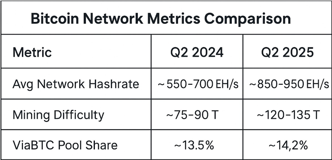
A mining strategy built with the ViaBTC Mining Guide should connect hardware efficiency, electricity price, pool payout rules, network difficulty, uptime, and coin economics before equipment runs. A 3.5 kW ASIC uses 84 kWh per day; at $0.06/kWh, power costs $5.04 daily or about $1,840 per year. If effective hashrate falls 5% below the rated figure, revenue can decline by roughly the same proportion before fixed operating expenses change. In 2026, miners should therefore compare cost per kWh, joules per unit of hashrate, accepted shares, fees, and payout structure rather than treating advertised hashrate as a complete profitability measure.

The ViaBTC Mining Guide is most useful when hardware selection starts with the mining algorithm rather than the coin price. Bitcoin ASICs built for SHA-256 cannot be reassigned to Scrypt mining simply because Litecoin economics improve. The same limitation applies in reverse. A miner should first identify compatible coins and pools, then compare expected output against electricity and equipment costs. If a 3.0 kW unit runs 24 hours, it consumes 72 kWh; moving from $0.05 to $0.09 per kWh raises daily electricity spending from $3.60 to $6.48, an 80% increase without adding any hashrate.

That cost difference makes efficiency more useful than headline speed when two machines are compared. A 100 TH/s unit drawing 3,000 W operates at 30 J/TH, while a 120 TH/s unit drawing 4,000 W uses about 33.3 J/TH. The second machine supplies 20% more hashrate but consumes 33.3% more electricity. At $0.07/kWh, their daily power bills are $5.04 and $6.72. A miner planning through 2026 should compare the extra daily output with the additional $1.68 power expense before paying more for the faster unit.

Rated hashrate describes machine capacity under specified conditions; pool-side accepted hashrate shows how much useful work reaches the pool. A machine advertised at 100 TH/s but averaging 96 TH/s effectively loses 4% of its expected productive capacity.

Pool-side performance therefore belongs in the financial model. Internet interruptions, thermal throttling, maintenance, rejected shares, firmware restarts, and power interruptions can reduce productive hours. At 98% uptime, a 30-day month provides about 705.6 operating hours instead of 720. At 95%, the figure falls to 684 hours. The difference is 21.6 hours of mining, or almost one full day, before rejected work is considered.

Once actual operating time is known, revenue estimates should use more than one market condition. Assume an ASIC produces $11 in gross daily mining revenue while electricity costs $5.50. The initial operating spread is $5.50. If gross revenue falls 15% to $9.35, the spread becomes $3.85, a 30% reduction. At a 30% revenue decline, gross income falls to $7.70 and the remaining spread contracts to $2.20. Hosting, maintenance, pool charges, cooling, and hardware cost still need to be paid from that amount.

A practical model can therefore test three operating cases rather than relying on a single calculator estimate:

Operating case	Gross daily revenue	Electricity	Other daily costs	Remaining amount
Base	$11.00	$5.50	$1.00	$4.50
Revenue -15%	$9.35	$5.50	$1.00	$2.85
Revenue -30%	$7.70	$5.50	$1.00	$1.20

The table also explains why electricity contracts deserve attention before hardware purchases. A machine consuming 3.5 kW needs 84 kWh each day and 30,660 kWh over 365 days at continuous operation. At $0.05/kWh, annual electricity is about $1,533; at $0.08, it reaches roughly $2,453. The $0.03 difference adds about $920 per machine each year. A 100-machine operation would face approximately $92,000 in additional annual electricity spending under the same consumption assumption.

Electricity alone does not show the complete operating cost, so hosting terms need the same treatment. A quoted rate may cover power while leaving setup, repair labor, deposits, cooling, administration, or minimum-contract periods outside the advertised number. If additional expenses add only $0.01 per kWh to the effective rate, the 3.5 kW example gains another $306.60 in annual cost. Across 50 machines, that becomes $15,330, enough to materially change a 2026 equipment budget.

Hardware purchase price should then be separated from daily operating cash flow. Suppose a miner costs $4,000 and generates $4.50 per day after electricity and routine operating expenses. A simple payback calculation produces about 889 days, or 2.44 years, assuming output and expenses never change. Mining conditions rarely remain unchanged for 889 days because network competition, transaction fees, coin prices, hardware efficiency, and equipment reliability can all move during that period.

Positive daily cash flow does not automatically recover the equipment purchase. A $4,000 machine producing $1.50 per day after operating expenses would need about 2,667 days, or 7.3 years, to recover its purchase price under unchanged conditions.

Network difficulty therefore needs to sit beside electricity in the model. A miner contributes a share of the network's computational work, so rising competing hashrate can reduce expected coin production per unit of miner hashrate. A planning sheet can test production at the current assumption, 10% lower, and 25% lower. Combining a 25% production reduction with a 10% increase in electricity price provides a more useful stress case than assuming 2026 conditions remain constant for several years.

Pool selection adds another layer because payout methods can change the timing and variability of mining income. Miners using the ViaBTC LTC Mining Pool can review pool information alongside their Scrypt hardware economics instead of evaluating the machine independently. For Litecoin-related mining, equipment compatibility, pool configuration, merged-mining arrangements where applicable, payout method, minimum payout conditions, and fee information should be checked against the pool's current published terms because service rules can change after 2026.

Payout structure matters most when operating bills are due on fixed dates. An operation paying $8,000 in monthly electricity cannot treat every mined coin as a long-term holding without maintaining separate working capital. One approach is to sell enough mining proceeds to cover the next billing cycle while retaining a defined portion. If monthly mining proceeds equal $12,000 and operating bills total $8,000, selling roughly 66.7% covers those bills before taxes and other obligations; retaining everything leaves the operator dependent on other cash.

That treasury choice should remain separate from the question of whether the machines themselves operate efficiently. If mined assets rise 20%, holding them can improve the final financial result, but appreciation does not repair inefficient hardware. A machine spending $7 per day to produce $6 of output loses $1 at the operating level regardless of whether previously mined coins later rise in price. Separating mining performance from asset-price exposure makes monthly records easier to interpret.

Daily records can stay compact. Record rated hashrate, pool-side hashrate, accepted shares, rejected shares, uptime, electricity consumption, mined units, and the reference market price used for accounting. If a 100 TH/s machine averages 97 TH/s for seven days, the 3% gap deserves investigation before a new profitability estimate is trusted. If the rejected-share rate moves from 0.5% to 2%, network connection, configuration, latency, or machine stability may deserve inspection.

The same records can establish operating thresholds. Assume a machine produces $8.50 per day while variable operating expenses are $6.00. It has a $2.50 daily cushion. A 20% revenue reduction lowers revenue to $6.80 and leaves only $0.80. A 30% reduction lowers revenue to $5.95, below the assumed variable expense. Predefined thresholds allow the operator to reduce power settings, move equipment, change compatible mining allocation, or stop a machine based on recorded numbers rather than short-term price movement.

Machine age can also affect those thresholds. If an older unit consumes 40 J/TH while a newer model provides comparable algorithmic work at 25 J/TH, the older machine uses 60% more energy per unit of hashrate. At low electricity prices both may operate economically, but the 40 J/TH unit reaches its operating-cost limit sooner when mining output falls. A mixed fleet should therefore be evaluated machine by machine rather than using one average electricity figure for every ASIC.

Cooling adds another measurable difference between rated and facility-level consumption. A 1 MW mining load does not always equal a 1 MW electricity bill for the entire site because ventilation, pumps, networking equipment, lighting, and other infrastructure also consume power. If supporting equipment adds 8%, a nominal 1 MW mining deployment requires about 1.08 MW at the facility level. Over 24 hours, that additional 80 kW represents 1,920 kWh beyond the miners themselves.

Facility capacity also limits expansion. Adding ten 3.5 kW miners requires 35 kW for the machines before supporting infrastructure is counted. With an 8% facility overhead assumption, the additional requirement approaches 37.8 kW. Running electrical infrastructure continuously near its rated limit may also conflict with local electrical standards, hosting rules, or equipment requirements, so usable capacity should come from the site's qualified electrical design rather than a simple nameplate calculation.

A mining plan works better when each assumption has a source and review date: electricity contract, ASIC specification, pool terms, measured uptime, actual accepted hashrate, and network data. A figure recorded in January 2026 should not automatically remain an input in August 2026.

Monthly review can then compare forecast numbers with measured results. If the model assumed 98% uptime but the fleet delivered 94%, a 30-day month lost about 28.8 more operating hours than planned. If power consumption averaged 3% above specification at the same time, both sides of the operating spread moved unfavorably. Updating the next month's forecast with measured data produces a more realistic estimate than continuing to use manufacturer specifications.

Capital expansion should use the same process. Before adding 20 machines, model their purchase cost, electrical capacity, 365-day power use, expected accepted hashrate, repair allowance, hosting terms, and revenue under at least two lower-output cases. Twenty 3.5 kW miners add 70 kW of mining load and approximately 613,200 kWh of annual consumption at continuous operation. At $0.06/kWh, electricity alone is about $36,792 per year before facility overhead.

Using the ViaBTC Mining Guide in this way turns pool information into operating inputs rather than reading material. Algorithm compatibility narrows the hardware choice; measured efficiency defines electricity exposure; pool statistics show delivered work; payout settings affect cash timing; monthly records show whether assumptions still match operations. A 5% difference in uptime, a $0.02/kWh change in electricity, or a 15% reduction in mining output can each materially alter a fleet's annual numbers, so every expansion or configuration change should be tested against measured costs before more capital is committed.